Pseudosection explorers tutorial

psexplorers provides several post-processing methods and visualizations of already constructed pseudosections. You can also create isopleths diagrams or do calculations along paths.

It provides four command-line scipts psgrid, psshow and psiso for quick visualizations. For options, check built-in help, e.g.:

$ psshow -h

To show pseudosection, you need to provide project file:

$ psshow -b /some/path/project.ptb

Using psexplorers in Python (or Jupyter notebook)

To access all options of psexplorer it is suggested to use Python API. You need to activate the pyps environment and run python interpreter:

$ conda activate pyps
$ python

To use psexplorer we need to import appropriate class, which contains most of the methods to work with pseudosection.

• PTPS class for P-T pseudosection constructed with ptbuilder

• TXPS class for T-X pseudosection constructed with txbuilder

• PXPS class for P-X pseudosection constructed with pxbuilder

All following commands must be executed in Python interpreter.

from pypsbuilder import PTPS

The second step is to create instance of pseudosection using existing project file.

pt = PTPS('/some/path/project.ptb')

We can check, whether the pseudosection already contains gridded calculations. If not, we can use calculate_composition method to calculate compositional variations on grid. The resulting data are stored in project file. Note that any new modifications of the project by pypsbuilder* will discard compositional variations on grid and must be calculated again.

if not pt.gridded:
    pt.calculate_composition(nx=50, ny=50)

Gridding 1/1: 100%|██████████| 2500/2500 [03:10<00:00, 13.12it/s]
Grid search done. 0 empty points left.

Visualize pseudosection

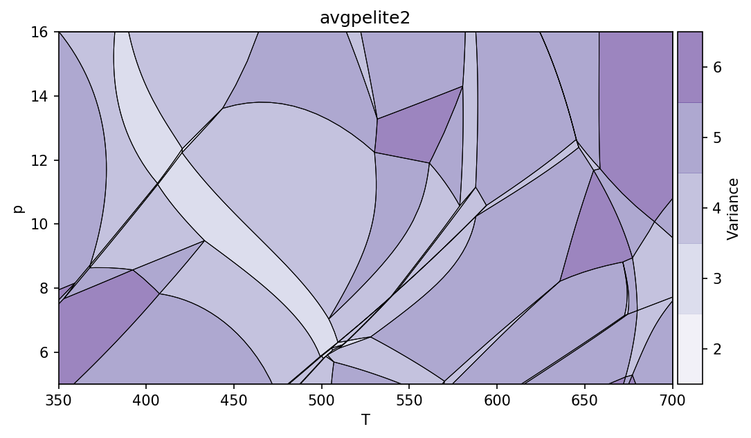
To show pseudosection, we can use show method

pt.show()

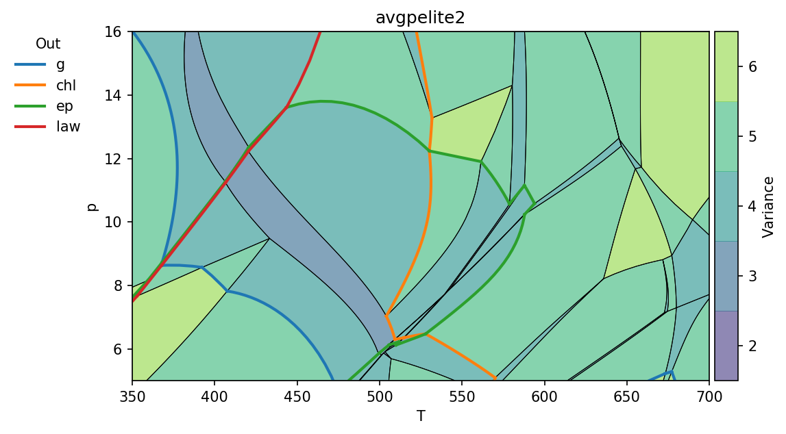
The keyword arguments cmap and out could be used to modify colormap and highlight zero mode lines across pseudosection.

pt.show(cmap='viridis', out=['g', 'chl', 'ep', 'law'])

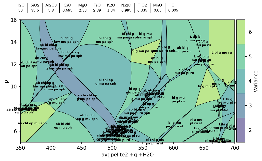
The keyword arguments bulk and label set whether the bulk composition is shown on figure and whether the fields are labeled by phases.

pt.show(cmap='viridis', bulk=True, label=True)

The pseudosection identify method could be used to identify stable assemblage for given p and T conditions. Note that returned key (Python frozenset) is used to identify stable assemblage in many PTPS methods.

key = pt.identify(550, 13)
print(key)

frozenset({'sph', 'pa', 'q', 'g', 'mu', 'H2O', 'bi'})

Access data and variables stored in project

The calculated data are usually accessed using stable assemblage key (see above). Theera are three groups of data stored 1) at invariant points, 2) along univariant lines and 3) on grid covering multivariate fields. To see data coverage and all available variables, you can use show_data method. When no variable (or expression) is provided, method will show available variables.

pt.show_data(key, 'g')

Missing expression argument. Available variables for phase g are:
mode x z m f xMgX xFeX xMnX xCaX xAlY xFe3Y H2O SiO2 Al2O3 CaO MgO FeO K2O Na2O TiO2 MnO O factor G H S V rho
Available end-members for g: kho gr alm py spss

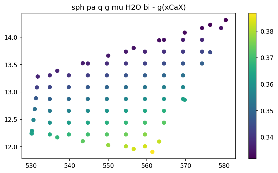
Once variable is provided, the all available data are shown.

pt.show_data(key, 'g', 'xCaX')

For data on the grid you can visualize them for all diagram in once using show_grid method.

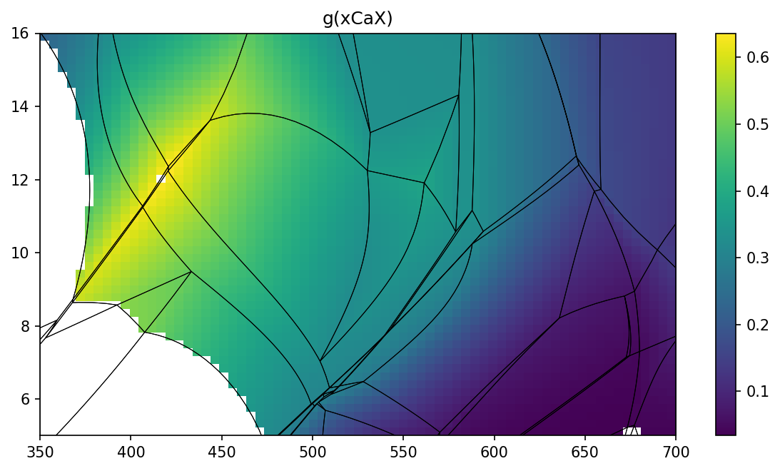
pt.show_grid('g', 'xCaX')

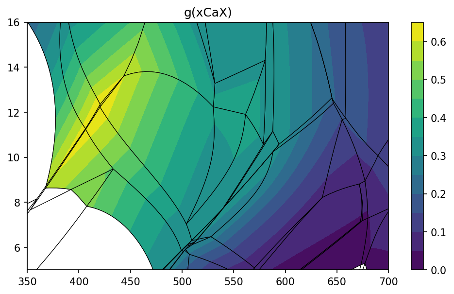
To create isopleths diagram you can use isopleths method. Note that contours are created separately for each stable assemblage allowing proper geometry of isopleths.

pt.isopleths('g', 'xCaX', N=14)

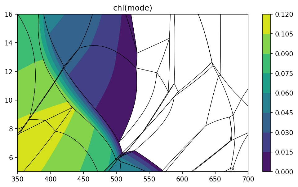
pt.isopleths('chl')

Missing expression argument. Available variables for phase chl are:
mode x y f m QAl Q1 Q4 xMgM1 xMnM1 xFeM1 xAlM1 xMgM23 xMnM23 xFeM23 xMgM4 xFeM4 xFe3M4 xAlM4 xSiT2 xAlT2 H2O SiO2 Al2O3 CaO MgO FeO K2O Na2O TiO2 MnO O factor G H S V rho
Available end-members for chl: ames mmchl ochl1 f3clin afchl ochl4 clin daph

pt.isopleths('chl', 'mode')

Calculations along PT paths

PTPS allows you to evaluate equilibria along user-defined PT path. PT path is defined by series of points (path is interpolated) and method collect_ptpath do actual calculations. It runs THERMOCALC with ptguesses obtained from existing calculations.

t = [380, 480, 580, 640, 500]
p = [7, 12, 15, 9, 5.5]
pa = pt.collect_ptpath(t, p)

Calculating: 100%|██████████| 100/100 [00:03<00:00, 25.86it/s]

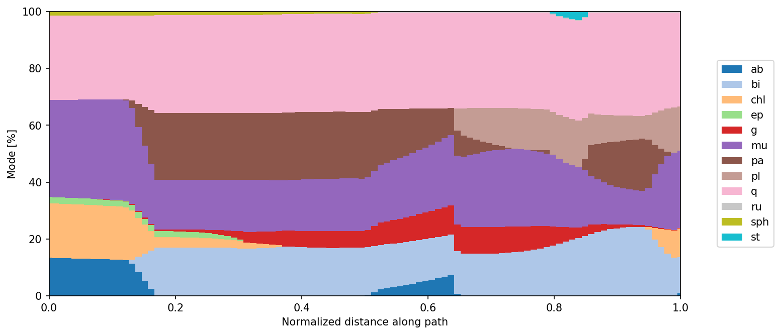
You can see phase modes along PT path using show_path_modes method.

pt.show_path_modes(pa, exclude=['H2O'])

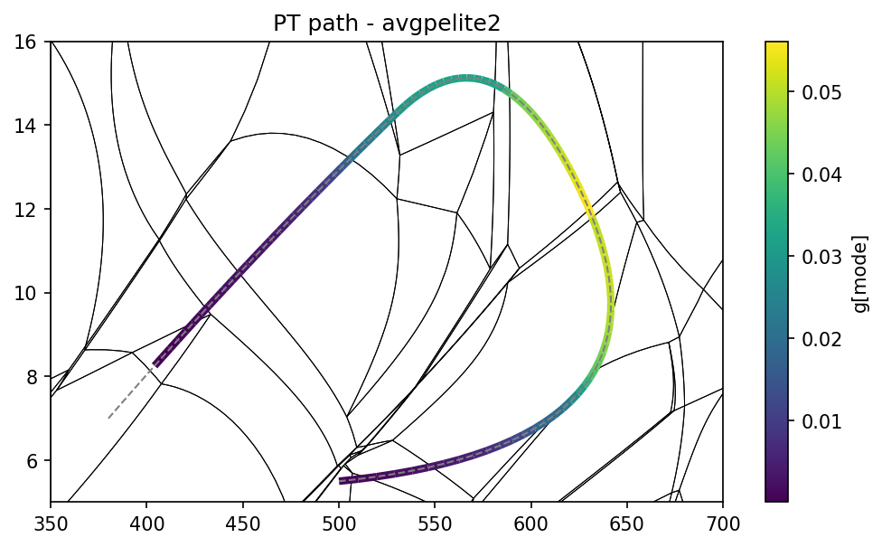
or show value of user-defined expression shown as colored strip on PT space.

pt.show_path_data(pa, 'g', 'mode')

Extra

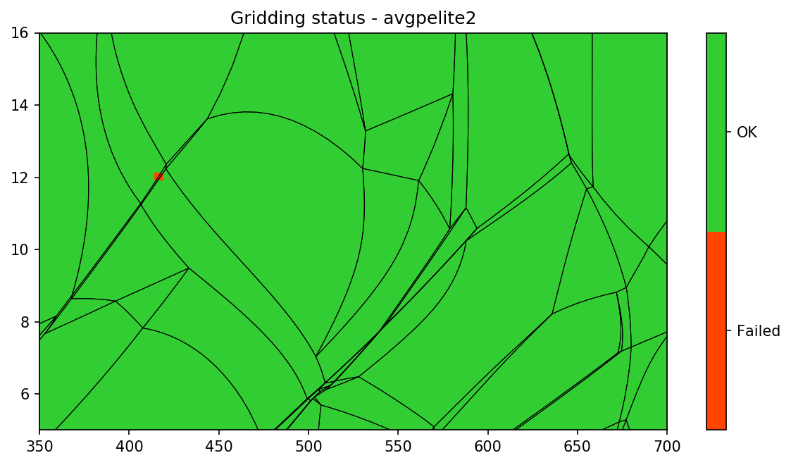
show_status method shows status of calculations on the grid. Possible failed calculations are shown.

pt.show_status()

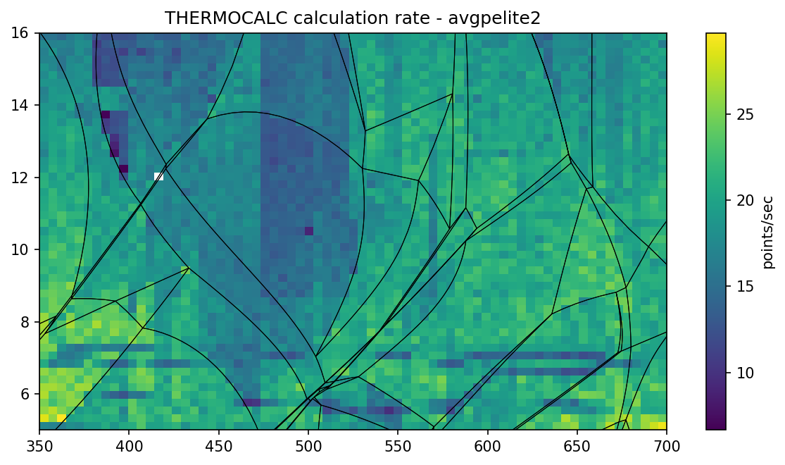
Do you want to know execution time of THERMOCALC on individual grid points? Check show_delta method.

pt.show_delta(pointsec=True)

For full description of Python API check: Python API.